13. Support Vector Machine (SVM)

• SVM is kind of Jack of All Trades for classifiers, because it is quite versatile and powerfull

• It does not save all training samples like NearestNeigbour method, but only the samples near the border of class boundaries.

• These boundary samples are called as support vectors.

• SVM works for high dimensional data and large sample sizes

• Can be used for both classification and regression

• Can be extended to nonlinear decision boundaries using kernels

13.1. Decision boundary

• SVM uses samples near the different clusters to define a decision boundary

• The boundary which maximises the marginal of the boundary will be selected

• THe support vectors definind the boundary will be stored

import numpy as np
import matplotlib.pyplot as plt
import seaborn as sns
sns.set()

from sklearn import datasets
from snippets import plotDB, DisplaySupportVectors

from sklearn.model_selection import train_test_split

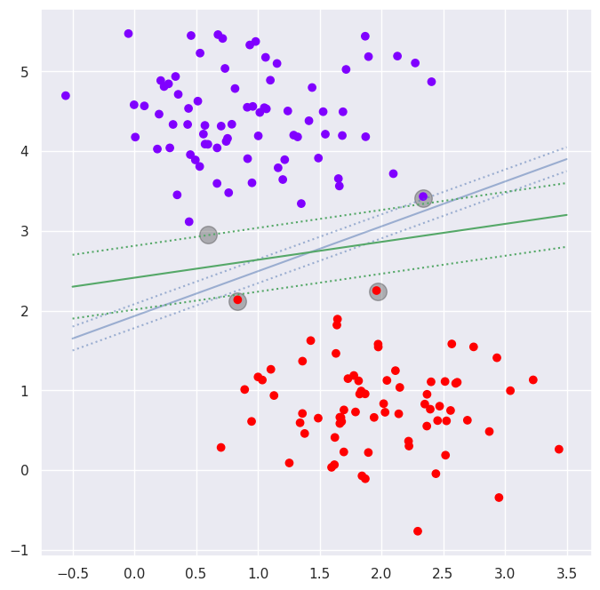
# Lets create a two-dimensional dataset containing two cluster centers
X,y=datasets.make_blobs(n_samples=200, centers=2, n_features=2, random_state=0, cluster_std=0.6)

# Now the dataset will be splitted randomly to training set and test set
X_train, X_test, y_train, y_test = train_test_split(X,y, test_size=0.25)

# Lets plot the data and optimal decision boundary with support vectors
a=plt.figure(figsize=(8,8))

plt.scatter([0.5965, 2.33479, 0.83645, 1.97], [2.9567, 3.4118, 2.11336, 2.23518],  s=200, c='k', alpha=0.3)

plt.scatter(X_train[:,0], X_train[:,1], c=y_train, cmap='rainbow')
ax=plt.gca()

# Plot decision boundaries
m=0.15; plt.plot([-0.5,3.5], [1.65,   3.9], 'b', alpha=0.5); plt.plot([-0.5,3.5], [1.65+m, 3.9+m], 'b:', alpha=0.5); plt.plot([-0.5,3.5], [1.65-m, 3.9-m], 'b:', alpha=0.5)
m=0.4; plt.plot([-0.5,3.5], [2.3, 3.2], 'g'); plt.plot([-0.5,3.5], [2.3+m, 3.2+m], 'g:'); plt.plot([-0.5,3.5], [2.3-m, 3.2-m], 'g:')

[<matplotlib.lines.Line2D at 0x706bbb4e2610>]

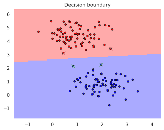
# Lets now try how actual linear SCV would work
from sklearn import svm, metrics
linsvc = svm.SVC(kernel='linear')
linsvc.fit(X_train, y_train)
plotDB(linsvc, X_train, y_train)
DisplaySupportVectors(X_train, y_train, linsvc)

print("Accurary in the trainint set..%f" % metrics.accuracy_score(y_true=y_train, y_pred=linsvc.predict(X_train)))
print("Accurary in the test set......%f" % metrics.accuracy_score(y_true=y_test, y_pred=linsvc.predict(X_test)))
print(linsvc)

Accurary in the trainint set..1.000000
Accurary in the test set......1.000000
SVC(kernel='linear')

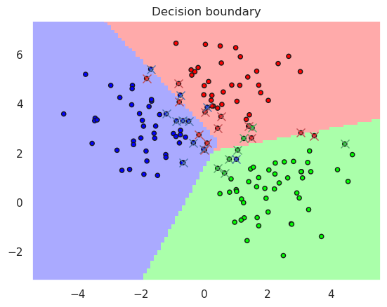
# Lets try slightly more complex case

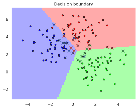
# Lets create a two-dimensional dataset containing three cluster centers
X,y=datasets.make_blobs(n_samples=200, centers=3, n_features=2, random_state=0, cluster_std=1.1)

# Now the dataset will be splitted randomly to training set and test set
X_train, X_test, y_train, y_test = train_test_split(X,y, test_size=0.25)

# Lets now try how actual linear SCV would work
from sklearn import svm
linsvc = svm.SVC(kernel='linear')
linsvc.fit(X_train, y_train)
plotDB(linsvc, X_train, y_train)

print("Accurary in the training set..%f" % metrics.accuracy_score(y_true=y_train, y_pred=linsvc.predict(X_train)))
print("Accurary in the test set......%f" % metrics.accuracy_score(y_true=y_test, y_pred=linsvc.predict(X_test)))
print(linsvc)

DisplaySupportVectors(X_train, y_train, linsvc)

Accurary in the training set..0.920000
Accurary in the test set......0.940000
SVC(kernel='linear')

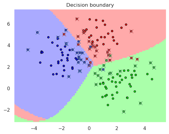
# Lets now try how actual linear SCV would work
Linsvc = svm.LinearSVC()
Linsvc.fit(X_train, y_train)
plotDB(Linsvc, X_train, y_train)

print("Accurary in the trainint set..%f" % metrics.accuracy_score(y_true=y_train, y_pred=Linsvc.predict(X_train)))
print("Accurary in the test set......%f" % metrics.accuracy_score(y_true=y_test, y_pred=Linsvc.predict(X_test)))
print(Linsvc)
DisplaySupportVectors(X_train, y_train, linsvc)

Accurary in the trainint set..0.926667
Accurary in the test set......0.920000
LinearSVC()

/home/petri/miniforge3/envs/octave/lib/python3.11/site-packages/sklearn/svm/_classes.py:31: FutureWarning: The default value of `dual` will change from `True` to `'auto'` in 1.5. Set the value of `dual` explicitly to suppress the warning.
  warnings.warn(

13.2. Kernel SVM

Linear kernel

# Lets now try Kernel SVM
rbfsvc = svm.SVC(kernel='rbf', gamma=0.1, C=0.5)  # gamma > 2 means overfitting, try eg 25 and 0.05
rbfsvc.fit(X_train, y_train)
plotDB(rbfsvc, X_train, y_train)

print("Accurary in the training set..%f" % metrics.accuracy_score(y_true=y_train, y_pred=rbfsvc.predict(X_train)))
print("Accurary in the test set......%f" % metrics.accuracy_score(y_true=y_test, y_pred=rbfsvc.predict(X_test)))
print(rbfsvc)
DisplaySupportVectors(X_train, y_train, rbfsvc)

Accurary in the training set..0.920000
Accurary in the test set......0.940000
SVC(C=0.5, gamma=0.1)

# Lets test the model with CV in higher nimensions

# Lets create a two-dimensional dataset containing three cluster centers
#X,y=datasets.make_blobs(n_samples=200, centers=5, n_features=3, random_state=0, cluster_std=2)
X,y=datasets.make_blobs(n_samples=200, centers=3, n_features=2, random_state=0, cluster_std=1.1)

# Now the dataset will be splitted randomly to training set and test set
X_train, X_test, y_train, y_test = train_test_split(X,y, test_size=0.25)

from sklearn.model_selection import cross_val_score
rbfsvc = svm.SVC(kernel='rbf', gamma=1, C=0.5)  # gamma > 2 means overfitting
scores = cross_val_score(rbfsvc, X_train, y_train, cv=5)
print("Mean CV score is %4.2f, all scores=" % (scores.mean()), scores)

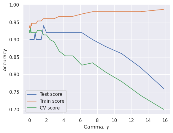
# CV can be put into loop to find optimal gamma value
gamma=np.logspace(-2,1.2,40)
test_score=np.zeros(len(gamma))
train_score=np.zeros(len(gamma))
cv_score=np.zeros(len(gamma))
for i in range(len(gamma)):
    rbfsvc = svm.SVC(kernel='rbf', gamma=gamma[i], C=0.5)
    rbfsvc.fit(X_train, y_train)
    train_score[i]=metrics.accuracy_score(y_train, rbfsvc.predict(X_train))
    test_score[i]=metrics.accuracy_score(y_test, rbfsvc.predict(X_test))
    cv_score[i] = cross_val_score(rbfsvc, X_train, y_train, cv=5).mean()
    

Mean CV score is 0.93, all scores= [0.93333333 0.96666667 0.86666667 0.9        0.96666667]

plt.plot(gamma, test_score, label="Test score")
plt.plot(gamma, train_score, label="Train score")
plt.plot(gamma, cv_score, label="CV score")
best_gamma=gamma[cv_score.argmax()]
print("Best gamma value is %f" % best_gamma)
rbfsvcbest = svm.SVC(kernel='rbf', gamma=best_gamma, C=0.5).fit(X_test, y_test)
plt.legend()
plt.xlabel('Gamma, $\gamma$')
plt.ylabel('Accuracy')
print("Accurary in the test set......%f" % metrics.accuracy_score(y_true=y_test, y_pred=rbfsvcbest.predict(X_test)))

Best gamma value is 0.037528
Accurary in the test set......0.920000

13.3. Non-linear SVM

• If the data described by \(p_i=[x_i, y_i]^T\) is not linearly separable, it can be made linearly separable by adding a new term, for example \(z_i=x_i^2 + y_i^2\)

• In this case, third dimension is introduced, and the linear classifier can work in the new three dimensional space \( p_i'=[x_i, y_i, z_i]^T \)

• SVM uses this kernel trick to separate non-linear cases

• The kernel functions include the dot product of two points in a suitable feature space. Thus defining a notion of similarity, with little computational cost even in very high-dimensional spaces.

• There are many kernel options, most common being

  • Polynomial kernel \(k(p_i, p_j) = (p_i \cdot p_j +1)^d\)

  • Gaussian kernel or Gaussian Radial Basis Function (RBF), shown below

  \[k(p_i, p_j) = \exp \left( - \frac{\Vert p_i-p_j \Vert^2}{2 \sigma^2} \right) \qquad k(p_i, p_j) = \exp ( - \gamma \Vert p_i-p_j \Vert^2) \]

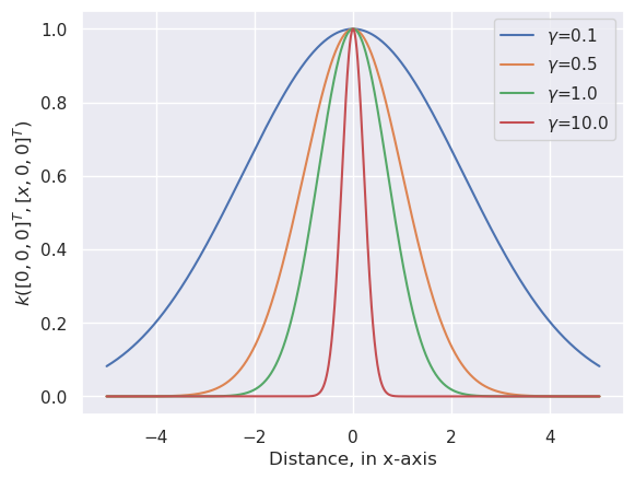
13.3.1. Illustration of RBF

• The following code plots the RBF when \(p_i\) is in origo and \(p_j\) moves along x-axis.

• In real case the RBF is N-dimensional, centered around a sample \(p_i\)

# Plot the radial basis functions (RBF) with different gamma values
xc=np.linspace(-5,5,1000)
for gamma in [0.1, 0.5, 1.0, 10.0, ]:
    r=np.exp(-gamma*xc**2)
    plt.plot(xc,r,label='$\gamma$=%3.1f' % (gamma))
plt.legend()
plt.xlabel('Distance, in x-axis')
plt.ylabel('$k([0,0,0]^T, [x,0,0]^T)$')

Text(0, 0.5, '$k([0,0,0]^T, [x,0,0]^T)$')

# Test with some example data.
# How to separate two classes with linear decision function
# This is one dimensional case, since the second dimension is dummy (only zeros)
x1=np.arange(-5,10)
x2=np.zeros(len(x1))
ytest=np.zeros(len(x1))
ytest[5:10]=1
plt.scatter(x1,x2,c=ytest, cmap='rainbow')

<matplotlib.collections.PathCollection at 0x706bb112f510>

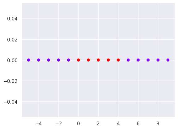
Solution: Use the 8th value as a support vector, and use RBF kernel to increase one more dimesion

# Import norm, which calculates || p1- p2 ||^2
from scipy.linalg import norm

# Define the RBF function
def rbf(p1, p2, gamma):
    return np.exp(-gamma*norm(p1-p2))

# Calculate the kernel value for all data points
for i in range(len(x1)):
    x2[i]=rbf(x1[7], x1[i], 0.5)
    
plt.scatter(x1,x2,c=ytest, cmap='rainbow')

# Mark almost optimal decision boundary as horizontal line
plt.axhline(0.3) 

<matplotlib.lines.Line2D at 0x706bb126ca10>

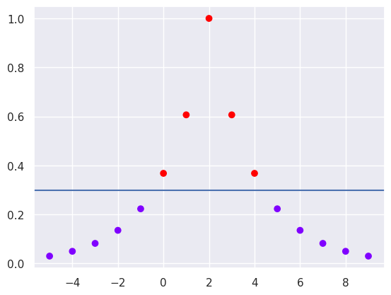
Now the classes are separable, but what is the optimal Gamma value?

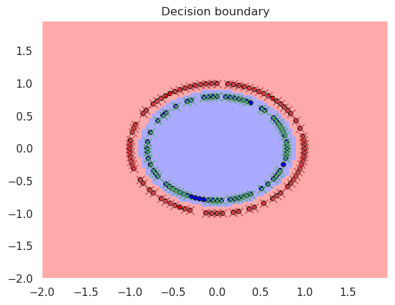
13.3.2. Testing RBF in circular data

Xc,yc=datasets.make_circles(n_samples=200)
X_train, X_test, y_train, y_test = train_test_split(Xc,yc, test_size=0.25)

rbfsvc = svm.SVC(kernel='rbf', gamma='scale')
rbfsvc.fit(X_train, y_train)

print("Accurary in the training set..%f" % metrics.accuracy_score(y_true=y_train, y_pred=rbfsvc.predict(X_train)))
print("Accurary in the test set......%f" % metrics.accuracy_score(y_true=y_test, y_pred=rbfsvc.predict(X_test)))
print(rbfsvc)
plotDB(rbfsvc, X_train, y_train)
DisplaySupportVectors(X_train, y_train, rbfsvc)

Accurary in the training set..1.000000
Accurary in the test set......1.000000
SVC()

rbfsvc = svm.SVC(kernel='rbf', gamma=0.5)
rbfsvc.fit(X_train, y_train)

print("Accurary in the training set..%f" % metrics.accuracy_score(y_true=y_train, y_pred=rbfsvc.predict(X_train)))
print("Accurary in the test set......%f" % metrics.accuracy_score(y_true=y_test, y_pred=rbfsvc.predict(X_test)))
print(rbfsvc)
plotDB(rbfsvc, X_train, y_train)
DisplaySupportVectors(X_train, y_train, rbfsvc)

Accurary in the training set..1.000000
Accurary in the test set......1.000000
SVC(gamma=0.5)

Read more from Understanding SVM

13.4. Summary

• SVM is good for high dimensional cases

• LinearSVC can include a regularization term L2, or L1

• KernelSVM can form non-linear decision boundaries

Cons

• SVM does not work so well for really big data sizes

• It has also problems if there is plenty of noise in the data, so that classes are overlapping