15. Regression and regularisation

• Regression is used when prediction a continuous dependent variable using one ore more independent variables.

• Most well known classical regression model is Ordinary Least Mean Squares (OLS) regression

• Classical regression is not working well when the number of features is large or when the data contains plenty of noise or the dependency is non-linear

• Application areas of classical regression can be extended by using regularisation

• Non-linear regression models are better when the dependency is not linear

• Many new regression models can also tolerate high dimensionality and non gaussian noise better than classical methods

• Some often used regression methods, also suited for non-linear dependencies and high-dimensional data are Suppor Vector Regression (SVR), Random Forest Regression (RFR), and Gradient Boosted Regression Trees (GBRT). See the discussion of usage of corresponding Support Vector Machine (SVM), Random Forest, and Gradient Boosting for classification, since their operating principles are the same for regression and classification.

• Recursive feature elimination/addition are useful methods for model optimisation and feature selection

15.1. Ordinary Least mean Squares (OLS) regression

• OLS using p-features \(x_i\) to predict variable \(y\).

• \(x_i\) are called as independent variables

• \(y\) is called as a dependent variable

• \(\beta_i\) are the model parameters

• \(\beta_0\) is the intersection, which is not always modeled

\[ \hat{y}_i = \beta_0 + \beta_1 x_{i,1} + \beta_2 x_{i,2} + \beta_3 x_{i,3} + \cdots + \beta_p x_{i,p} + \epsilon_i \]

Cost function to be minimized (square error):

\[ Obj(\Theta) = L(\Theta) = \sum_{i=1}^{n} (y_i - \sum_{j=1}^p \beta_j x_{ij})^2 \]

This Classic regression, usually the first choice to be tested. It Does not work well when p is large and when the training data contains plenty of noise

The prediction with the model is the following:

\[ \hat{y} = \beta_0 + \beta_1 x_1 + \beta_2 x_2, ..., \beta_n x_n + \epsilon \]

In 1-dimensional case, the regression is simply

\[ \hat{y} = \beta_0 + \beta_1 x + \epsilon, \]

where \(\beta_1\) is the reciprocal and \(\beta_0\) is the constant (the y-axis crossing point) and \(\epsilon\) is the prediction error. The optimal solution is when the squared sum of error (Loss function, \(L()\)) between predicted and true values is minimized:

\[ L(\beta) = \sum_{i=1}^{n} (y_i - \hat{y})^2 \]

The linear regression has a well known solution, which can be calculated very efficiently (closed form):

\[ \beta = (\mathbf{X}^T\mathbf{X})^{-1}\mathbf{X}^T Y, \]

Where \(\mathbf{X}\) is a design matrix containing data samples in rows, and variables in columns. It is also called as design matrix, at it was shown in the top of this section.

15.2. The fitness of a regression model

The fitness of a regression model is often estimated using coefficient of determination (\(R^2\)) or Root Mean Square Error of prediction (RMSE).

15.2.1. Coefficient of determination, \(R^2\)

The coefficient of determination, \(R^2\), defines how large proportion of the variance in \(y\) is explained by the model. \(R^2\) is zero if the model cannot predict anything and it is 1 when the model fit is perfect.

\[ R^2 = 1- \frac{\mathrm{var(residual)}}{\mathrm{var}(y)} = 1- \frac{\Sigma_{i=1}^{n} (y_i - \hat{y}_i)^2}{\Sigma_{i=1}^{n} (y_i - \bar{y})^2} \]

For Ordinary Least mean Squares regression models (OLS) it is the same as the square of the Pearson correlation coefficient.

\[ R^2 = \rho^2 \]

15.2.2. Root Mean Square Error, RMSE

RMSE, is another often used measure for model fitness. RMSE shows the average prediction error in the same units and scale than \(y\).

\[ \mathrm{RMSE} = \sqrt{ \left( \frac{\sum_{i=i}^{n} (y_i - \hat{y}_i)^2}{n} \right) } \]

15.3. Regularization and model simplicication

Ockham - from a manuscipt of Ockham’s Summa Logicae, MS Gonville and Caius College, Cambridge, 464/571, fol. 69r

“Simpler solutions are more likely to be correct than complex ones”

William of Ockham

Finding a model which fits to the data is not necessarily optimal. It may be unnecessary complex, which can cause problems in:

• Generalization: too complex models may have unnecessary complex decision boundary or use redundant or unimportant variables in a regression model, which are producing noise to the model. The model may event fit to the noise in the training data, which is not repeated similarly in new samples.

• Explainability: A complex model is difficult to understand, explain and believe.

• Stability: Too complex model may have problems in converging in noisy training data and also the prediction can be too noise sensitive

• Unnecessary high dimensionality means costs in recording, transferring, storing and processing data

Therefore it is important to use means for simplifying data and making the models more stable.

15.3.1. L2 regularization, Ridge regression

\[ Obj(\Theta) = \underbrace{\sum_{i=1}^{n} (y_i - \sum_{j=1}^p \beta_j x_{ij})^2}_{L(\Theta)} + \underbrace{\lambda \sum_{j=1}^p \beta_j^2}_{\Omega(\Theta)} \]

• Regularization term, \(\Omega(\Theta)\), makes it suitable for higher dimensional data

• Minimal unbiased estimator in certain cases

• Can be solved in closed form

• All coefficients are always kept -> Does not provide a parsimonious model

---

Hoerl, Arthur E., ja Robert W. Kennard. ”Ridge Regression: Biased Estimation for Nonorthogonal Problems”. Technometrics 12, nro 1 (1. Feb 1970): 55–67. https://doi.org/10.1080/00401706.1970.10488634.

15.3.2. L1 regularization, LASSO

\[ Obj(\Theta) = \underbrace{\sum_{i=1}^{n} (y_i - \sum_{j=1}^p \beta_j x_{ij})^2}_{L(\Theta)} + \lambda \sum_{j=1}^p |\beta_j| \]

• L1 regularization tends to lead solutions where many coefficients, \(\beta_i\) will be zeros -> sparse model.

• Only iterative solutions are available, but for example Least Angle Regression (LARS) is fast method for finding LASSO solution

• Will saturate if p>n, and select at maximum n feautures

• in cases where n>p and high correlation between predictors, L1 is worse than L2

---

Tibshirani, Robert. ”Regression Shrinkage and Selection Via the Lasso”. Journal of the Royal Statistical Society: Series B (Methodological) 58, nro 1 (1996): 267–88. https://doi.org/10.1111/j.2517-6161.1996.tb02080.x.

15.3.3. Elastic nets

\[ Obj(\Theta) = \underbrace{\sum_{i=1}^{n} (y_i - \sum_{j=1}^p \beta_j x_{ij})^2}_{L(\Theta)} + \lambda \sum_{j=1}^p \left( (1-\alpha) \beta_i^2 + \alpha |\beta_j| \right) \]

• Elastic net can perform like Rigde regression, when \(\alpha\)=0 or like LASSO when \(\alpha\)=1

• For suitable value of, \(\alpha\), elastic net will also produce sparse model, but it does not saturate to in cases when n<p like LASSO.

• Can tolerate correlation between predictors

• Can be computed interatively quite efficiently

Zou, Hui, ja Trevor Hastie. ”Regularization and variable selection via the elastic net”. Journal of the Royal Statistical Society: Series B (Statistical Methodology) 67, nro 2 (1. April 2005): 301–20. https://doi.org/10.1111/j.1467-9868.2005.00503.x.

15.3.4. Gradient Tree Boosting

• Also called as Gradient Boosted Regression Trees (GBRT)

• The GBRT has similar formal loss function and measure for complexity as linear regrssion

\[Obj(\Theta) = \underbrace{L(\Theta)}_{Training Loss} + \underbrace{\Omega(\Theta)}_{Regularization}\]

15.4. Coding examples

Pay attention especially for these rows

• Build the model:

    model = Model(<model parameters>).fit(X,y)

• Validate the model with R2 score in testing set and calculating Cross validation R2 score or R2 score and finaly for a separate testing set:

    model.score(X,y) model.cross_val_score(model, X, y, cv=5).mean() model.score(X_test, y_test)

• Variable selection:

    sfm = SelectFromModel(model, threshold=0.3) cross_val_score(model, sfm.transform(X), y, cv=5).mean() model.score(sfm.transform(X),y)

• Recursive feature selection

    rfe = RFE(estimator=model, n_features_to_select=1, step=1)

15.4.1. Boston house prizes example

Can the house prizes be predicted? Which parameters affect most to the house prizes?

    - CRIM     per capita crime rate by town
    - ZN       proportion of residential land zoned for lots over 25,000 sq.ft.
    - INDUS    proportion of non-retail business acres per town
    - CHAS     Charles River dummy variable (= 1 if tract bounds river; 0 otherwise)
    - NOX      nitric oxides concentration (parts per 10 million)
    - RM       average number of rooms per dwelling
    - AGE      proportion of owner-occupied units built prior to 1940
    - DIS      weighted distances to five Boston employment centres
    - RAD      index of accessibility to radial highways
    - TAX      full-value property-tax rate per \$10,000
    - PTRATIO  pupil-teacher ratio by town
    - B        1000(Bk - 0.63)^2 where Bk is the proportion of blacks by town
    - LSTAT    % lower status of the population
    - MEDV     Median value of owner-occupied homes in $1000's

import numpy as np
from sklearn.datasets import load_boston
from sklearn.linear_model import LinearRegression, Ridge, Lasso, ElasticNet, LassoCV, ElasticNetCV
from sklearn.feature_selection import SelectFromModel
import seaborn as sns
from sklearn.model_selection import cross_val_score
import pandas as pd
from sklearn.preprocessing import StandardScaler

scaler = StandardScaler()

boston=load_boston()
# Scaling is not necessary, but can be done
X= scaler.fit_transform(boston['data'])
Xorig= boston['data']
y= boston['target']
Boston = pd.DataFrame(data=X, columns=boston['feature_names'])
Boston['target'] = y
print(Boston.shape)
Boston.head()

(506, 14)

/home/petri/venv/python3/lib/python3.9/site-packages/sklearn/utils/deprecation.py:87: FutureWarning: Function load_boston is deprecated; `load_boston` is deprecated in 1.0 and will be removed in 1.2.

    The Boston housing prices dataset has an ethical problem. You can refer to
    the documentation of this function for further details.

    The scikit-learn maintainers therefore strongly discourage the use of this
    dataset unless the purpose of the code is to study and educate about
    ethical issues in data science and machine learning.

    In this special case, you can fetch the dataset from the original
    source::

        import pandas as pd
        import numpy as np


        data_url = "http://lib.stat.cmu.edu/datasets/boston"
        raw_df = pd.read_csv(data_url, sep="\s+", skiprows=22, header=None)
        data = np.hstack([raw_df.values[::2, :], raw_df.values[1::2, :2]])
        target = raw_df.values[1::2, 2]

    Alternative datasets include the California housing dataset (i.e.
    :func:`~sklearn.datasets.fetch_california_housing`) and the Ames housing
    dataset. You can load the datasets as follows::

        from sklearn.datasets import fetch_california_housing
        housing = fetch_california_housing()

    for the California housing dataset and::

        from sklearn.datasets import fetch_openml
        housing = fetch_openml(name="house_prices", as_frame=True)

    for the Ames housing dataset.
    
  warnings.warn(msg, category=FutureWarning)

	CRIM	ZN	INDUS	CHAS	NOX	RM	AGE	DIS	RAD	TAX	PTRATIO	B	LSTAT	target
0	-0.419782	0.284830	-1.287909	-0.272599	-0.144217	0.413672	-0.120013	0.140214	-0.982843	-0.666608	-1.459000	0.441052	-1.075562	24.0
1	-0.417339	-0.487722	-0.593381	-0.272599	-0.740262	0.194274	0.367166	0.557160	-0.867883	-0.987329	-0.303094	0.441052	-0.492439	21.6
2	-0.417342	-0.487722	-0.593381	-0.272599	-0.740262	1.282714	-0.265812	0.557160	-0.867883	-0.987329	-0.303094	0.396427	-1.208727	34.7
3	-0.416750	-0.487722	-1.306878	-0.272599	-0.835284	1.016303	-0.809889	1.077737	-0.752922	-1.106115	0.113032	0.416163	-1.361517	33.4
4	-0.412482	-0.487722	-1.306878	-0.272599	-0.835284	1.228577	-0.511180	1.077737	-0.752922	-1.106115	0.113032	0.441052	-1.026501	36.2

# Ordinary Linear Regression First
lr=LinearRegression().fit(X,y)
yhat=lr.predict(X)

# Cross_val_score and score are coefficient of determinations, R^2
RsquaredCV=cross_val_score(lr, X, y, cv=5).mean()
RsquaredTR=lr.score(X,y)

sns.regplot(x=y,y=yhat, line_kws={"color": "red"})
plt.xlabel('True price')
plt.ylabel('Predicted price')
plt.title('Comparison of two-feature model, $R^2$=%3.2f' % RsquaredCV)
print("CV score..........", RsquaredCV)
print("Training score....", RsquaredTR)

CV score.......... 0.3532759243958824
Training score.... 0.7406426641094095

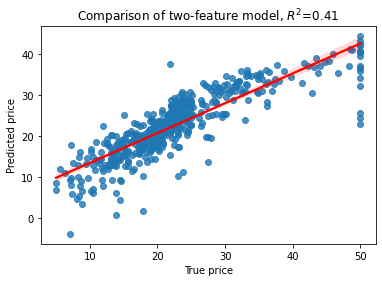
# Then L2 regularized Ridge Regression
rr=Ridge(alpha=12).fit(X,y)
yhat=rr.predict(X)
RsquaredCV=cross_val_score(rr, X, y, cv=5).mean()
RsquaredTR=rr.score(X,y)

sns.regplot(x=y,y=yhat, line_kws={"color": "red"})
plt.xlabel('True price')
plt.ylabel('Predicted price')
plt.title('Comparison of two-feature model, $R^2$=%3.2f' % RsquaredCV)
print("CV score..........", RsquaredCV)
print("Training score....", RsquaredTR)

CV score.......... 0.41282930221133507
Training score.... 0.7394797644213642

# L1 regularized Lasso Regerssion
la=Lasso(alpha=0.1).fit(X,y)
yhat=la.predict(X)
RsquaredCV=cross_val_score(la, X, y, cv=5).mean()
RsquaredTR=la.score(X,y)

sns.regplot(x=y, y=yhat, line_kws={"color": "red"})
plt.xlabel('True price')
plt.ylabel('Predicted price')
plt.title('Comparison of two-feature model, $R^2$=%3.2f' % RsquaredCV)
print("CV score..........", RsquaredCV)
print("Training score....", RsquaredTR)

CV score.......... 0.40368942076383674
Training score.... 0.7353093744353656

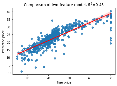
# L2 + L1 regularized Elastic Net
en=ElasticNet(alpha=0.5, l1_ratio=0.1).fit(X,y)
yhat=en.predict(X)
RsquaredCV=cross_val_score(en, X, y, cv=5).mean()
RsquaredTR=en.score(X,y)

sns.regplot(x=y, y=yhat, line_kws={"color": "red"})
plt.xlabel('True price')
plt.ylabel('Predicted price')
plt.title('Comparison of two-feature model, $R^2$=%3.2f' % RsquaredCV)
print("CV score..........", RsquaredCV)
print("Training score....", RsquaredTR)

CV score.......... 0.4497867885311699
Training score.... 0.6877704284092927

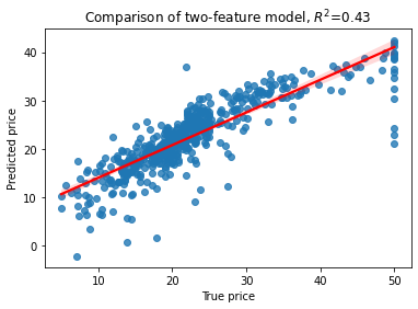
# Lets use Elastic Net for selecting the most relevant features
#model = LassoCV(cv=5)
model = ElasticNetCV(cv=5).fit(X,y)
yhat=model.predict(X)
RsquaredCV=cross_val_score(model, X, y, cv=5).mean()
RsquaredTR=en.score(X,y)
 
sns.regplot(x=y, y=yhat, line_kws={"color": "red"})
plt.xlabel('True price')
plt.ylabel('Predicted price')
plt.title('Comparison of two-feature model, $R^2$=%3.2f' % RsquaredCV)
print("CV score..........", RsquaredCV)
print("Training score....", RsquaredTR)

print("alpha=%f, L1-ratio=%f" % (model.alpha_, model.l1_ratio))

CV score.......... 0.4269743096160285
Training score.... 0.6877704284092927
alpha=0.192143, L1-ratio=0.500000

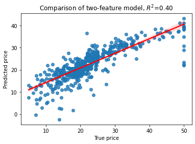
# Lets use Elastic Net for selecting the most relevant features
#model = LassoCV(cv=5)
model = ElasticNetCV(cv=5)

sfm = SelectFromModel(model, threshold=1.5)
sfm.fit(X, y)

print(sfm.transform(X).shape)
print("Selected variables are", sfm.transform([boston['feature_names'], boston['feature_names']])[0])
        

(506, 4)
Selected variables are ['RM' 'DIS' 'PTRATIO' 'LSTAT']

model.fit(sfm.transform(X), y)
yhat=model.predict(sfm.transform(X))
RsquaredCV=cross_val_score(model, sfm.transform(X), y, cv=5).mean()
RsquaredTR=model.score(sfm.transform(X),y)

sns.regplot(x=y,y=yhat, line_kws={"color": "red"})
plt.xlabel('True price')
plt.ylabel('Predicted price')
plt.title('Comparison of two-feature model, $R^2$=%3.2f' % RsquaredCV)
print("CV score..........", RsquaredCV)
print("Training score....", RsquaredTR)

Rsquared=sum((yhat-np.mean(y))**2)/sum((y-np.mean(y))**2)

CV score.......... 0.40003779874768786
Training score.... 0.6879971162429187

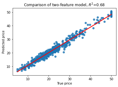
15.5. Gradient tree regression

from sklearn.ensemble import GradientBoostingRegressor
from sklearn.model_selection import cross_val_score

#est = GradientBoostingRegressor(n_estimators=50, learning_rate=0.1,
#                                max_depth=2, random_state=0, loss='ls')
est = GradientBoostingRegressor(max_features=3)
est.fit(X, y)
yhat=est.predict(X)
RsquaredCV=cross_val_score(est, X, y, cv=5).mean()
RsquaredTR=est.score(X,y)

sns.regplot(x=y,y=yhat, line_kws={"color": "red"})
plt.xlabel('True price')
plt.ylabel('Predicted price')
plt.title('Comparison of two-feature model, $R^2$=%3.2f' % RsquaredCV)
print("CV score..........", RsquaredCV)
print("Training score....", RsquaredTR)

CV score.......... 0.6835129936048598
Training score.... 0.9681703971776361

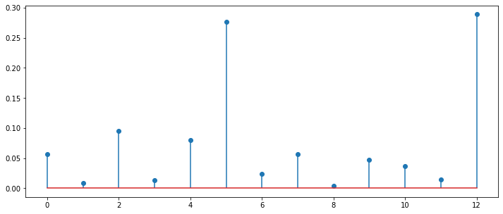
# Plot the importance of each feature
plt.figure(figsize=(12,5))
#Rsquared=sum((yhat-np.mean(y))**2)/sum((y-np.mean(y))**2)
i=range(len(boston.feature_names))
plt.stem(est.feature_importances_)
ax=plt.gca()
#ax.set_xticklabels(boston.feature_names);

for i in range(len(boston.feature_names)):
    print("%2d %8s=%5.2f" % (i,boston.feature_names[i], est.feature_importances_[i]))

 0     CRIM= 0.06
 1       ZN= 0.01
 2    INDUS= 0.09
 3     CHAS= 0.01
 4      NOX= 0.08
 5       RM= 0.28
 6      AGE= 0.02
 7      DIS= 0.06
 8      RAD= 0.00
 9      TAX= 0.05
10  PTRATIO= 0.04
11        B= 0.01
12    LSTAT= 0.29

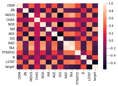
sns.heatmap( ))
Boston.corr()

	CRIM	ZN	INDUS	CHAS	NOX	RM	AGE	DIS	RAD	TAX	PTRATIO	B	LSTAT	target
CRIM	1.000000	-0.200469	0.406583	-0.055892	0.420972	-0.219247	0.352734	-0.379670	0.625505	0.582764	0.289946	-0.385064	0.455621	-0.388305
ZN	-0.200469	1.000000	-0.533828	-0.042697	-0.516604	0.311991	-0.569537	0.664408	-0.311948	-0.314563	-0.391679	0.175520	-0.412995	0.360445
INDUS	0.406583	-0.533828	1.000000	0.062938	0.763651	-0.391676	0.644779	-0.708027	0.595129	0.720760	0.383248	-0.356977	0.603800	-0.483725
CHAS	-0.055892	-0.042697	0.062938	1.000000	0.091203	0.091251	0.086518	-0.099176	-0.007368	-0.035587	-0.121515	0.048788	-0.053929	0.175260
NOX	0.420972	-0.516604	0.763651	0.091203	1.000000	-0.302188	0.731470	-0.769230	0.611441	0.668023	0.188933	-0.380051	0.590879	-0.427321
RM	-0.219247	0.311991	-0.391676	0.091251	-0.302188	1.000000	-0.240265	0.205246	-0.209847	-0.292048	-0.355501	0.128069	-0.613808	0.695360
AGE	0.352734	-0.569537	0.644779	0.086518	0.731470	-0.240265	1.000000	-0.747881	0.456022	0.506456	0.261515	-0.273534	0.602339	-0.376955
DIS	-0.379670	0.664408	-0.708027	-0.099176	-0.769230	0.205246	-0.747881	1.000000	-0.494588	-0.534432	-0.232471	0.291512	-0.496996	0.249929
RAD	0.625505	-0.311948	0.595129	-0.007368	0.611441	-0.209847	0.456022	-0.494588	1.000000	0.910228	0.464741	-0.444413	0.488676	-0.381626
TAX	0.582764	-0.314563	0.720760	-0.035587	0.668023	-0.292048	0.506456	-0.534432	0.910228	1.000000	0.460853	-0.441808	0.543993	-0.468536
PTRATIO	0.289946	-0.391679	0.383248	-0.121515	0.188933	-0.355501	0.261515	-0.232471	0.464741	0.460853	1.000000	-0.177383	0.374044	-0.507787
B	-0.385064	0.175520	-0.356977	0.048788	-0.380051	0.128069	-0.273534	0.291512	-0.444413	-0.441808	-0.177383	1.000000	-0.366087	0.333461
LSTAT	0.455621	-0.412995	0.603800	-0.053929	0.590879	-0.613808	0.602339	-0.496996	0.488676	0.543993	0.374044	-0.366087	1.000000	-0.737663
target	-0.388305	0.360445	-0.483725	0.175260	-0.427321	0.695360	-0.376955	0.249929	-0.381626	-0.468536	-0.507787	0.333461	-0.737663	1.000000

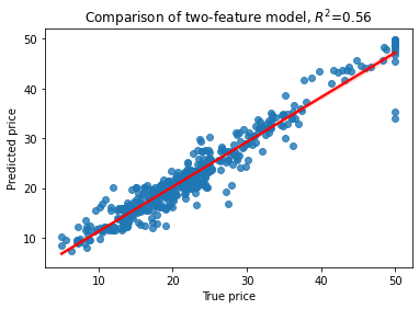
selected=est.feature_importances_.argsort()[-1:-4:-1]
print(selected)

Xs=X[:,selected]
print(Xs.shape)

ests = GradientBoostingRegressor()
ests.fit(Xs, y)
yhat=ests.predict(Xs)
RsquaredCV=cross_val_score(ests, Xs, y, cv=5).mean()
RsquaredTR=ests.score(Xs,y)

sns.regplot(x=y, y=yhat, line_kws={"color": "red"})
plt.xlabel('True price')
plt.ylabel('Predicted price')
plt.title('Comparison of two-feature model, $R^2$=%3.2f' % RsquaredCV)
print("CV score..........", RsquaredCV)
print("Training score....", RsquaredTR)
ests

[12  5  2]
(506, 3)
CV score.......... 0.5625462771221375
Training score.... 0.9304873266368128

GradientBoostingRegressor()

15.6. Recursive feature elimination

An example of familiar digits classification

from sklearn.svm import SVC
from sklearn.datasets import load_digits
from sklearn.feature_selection import RFE
import matplotlib.pyplot as plt

# Load the digits dataset
digits = load_digits()
X = digits.images.reshape((len(digits.images), -1))
y = digits.target

# Create the RFE object and rank each pixel
svc = SVC(kernel="linear", C=1)
rfe = RFE(estimator=svc, n_features_to_select=1, step=1)
rfe.fit(X, y) 

RFE(estimator=SVC(C=1, kernel='linear'), n_features_to_select=1)

ranking = rfe.ranking_.reshape(digits.images[0].shape)

# Plot pixel ranking
plt.matshow(ranking, cmap=plt.cm.Blues)
plt.colorbar()
plt.title("Ranking of pixels with RFE")
plt.show()

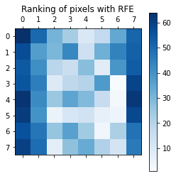
rfe.ranking_.reshape(digits.images[0].shape)

array([[64, 50, 31, 23, 10, 17, 34, 51],
       [57, 37, 30, 43, 14, 32, 44, 52],
       [54, 41, 19, 15, 28,  8, 39, 53],
       [55, 45,  9, 18, 20, 38,  1, 59],
       [63, 42, 25, 35, 29, 16,  2, 62],
       [61, 40,  5, 11, 13,  6,  4, 58],
       [56, 47, 26, 36, 24,  3, 22, 48],
       [60, 49,  7, 27, 33, 21, 12, 46]])

15.7. Summary

• Classical regression is simple and well understood, and is a good model, when its conditions are met

  • The number of features is much less than number of samples

  • There is not too much noise in the data

  • The linear model is sufficient

  • Data needs to be normalized before use

  • Categorical data is not well supported, at least needs to be converted to numerical for example using one hot encoding

• Regularisation includes many methods for balancing the trade off between model complexity and prediction error which prevents against over-fitting of the model

  • Regularization is often used in two forms: L2-regularization minimises the squared sum of model parameters, L1-regularization minimises the absolute sum of the model parameters.

• Non-linear regression models SVR, RFR, GBRT extend the regression to non-linear problems

• Ensemble models include a bag (parallel) or boosted (serial) combination of many simple models, which are randomized (bag) or boosted versions of simple regressors

  • Extratrees and Gradient Boosted Regression Trees can also use categorical data directly and they do not need the normalization of data

• Recursive feature elimination (RFE)/addition are useful methods for model optimisation and feature selection

• The feature importances measure in RF and GBTR models provides a clue for the importance of features

• R2-score and RMSE are typical measures for model performance